Genetic Algorithm Form

The Genetic Algorithm Optimization form is created by clicking the Optimization button on the main form with the adjacent pulldown menu set to Genetic Algorithm. This form employs a genetic algorithm (GA) to explore the design space. When the form is opened, no other window of Attune can be made active. This prevents the initial design shown on the optimization form from being inconsistent with the rest of Attune. The design and state variable summary tables on the Genetic Algorithm form can be used to track the current state of the design.

The Design Variable Summary table has a few extra columns here. The fourth and fifth columns of the Design Variable Summary table are the Lower Bound and Upper Bound for the design variables. Initially, these values correspond to the effective bounds based on the bounds and limits on the Design Variable form. These effective bounds can be edited in the table. However, the effect will be local to the genetic algorithm. That is, modified bounds will be used for the optimization, but the bounds will revert once the Genetic Algorithm Optimization form is closed. Obviously, the active design variables must have valid effective bounds for this optimization method.

The sixth column from the left of the table is the Number of Bits used to discretize the design space for a particular design variable. The column to the right of that shows the Resolution of the discretization used (see the Theory section on genetic algorithm for more details). The user can change the number of bits used for the discretization editing the values in the table directly and by using the copy and paste functionality available on the table’s contextual menu.

The penultimate column on the right of the table, Minimum Delta, shows the smallest possible change in the design variable due to discretization. In other words, if the minimum delta is 0.00039, the genetic algorithm cannot produce a design in which the design variable changes by less than 0.00039. A design change of 0.0 is not possible. Because 0.0 design change is often not an element of the discrete design space, the Toggle Zero dv button shifts the range of the selected design variable(s) so that 0.0 design change is among the discrete design possibilities.

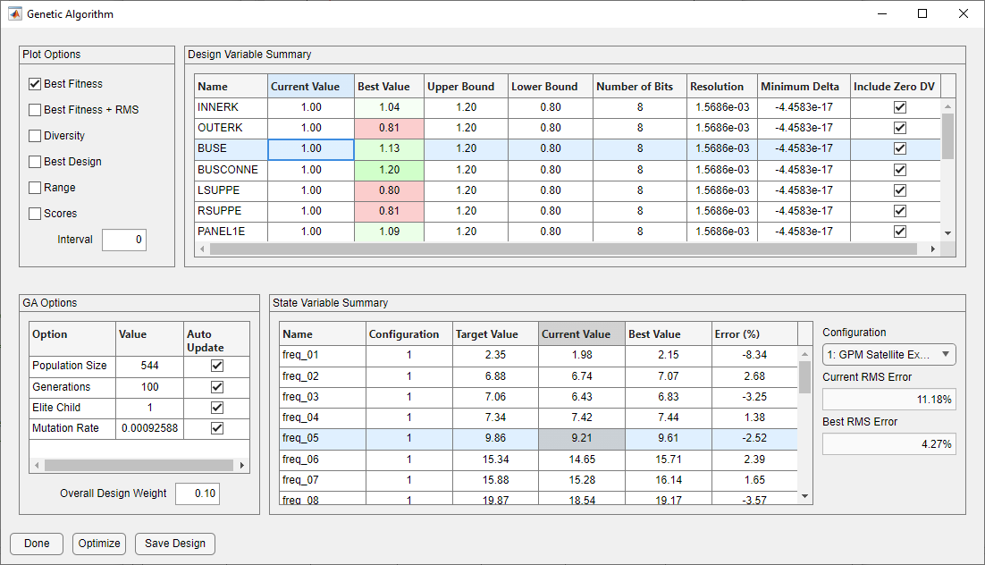
Genetic Algorithm Form

The table in the lower left of the form controls the operation of the genetic algorithm. The first field, Population Size, determines the size of the population at each iteration. The default is four times the total length of the bit string. The bit string is the method used in the genetic algorithm to describe the design. The length of the bit string is equal to the sum of the number of bits used for all active design variables.

The next field, Generations, is the number of generations; it controls how many iterations will be performed during the optimization. This is currently the only method for automatically terminating the genetic algorithm.

The Elite Child field refers to the technique of taking the best design(s) directly into the next generation, without crossover or mutation. Elite children are not necessary, but having elite children is the only way to guarantee that the overall error never increases during iteration. This value corresponds to the number of elite children to bring to the subsequent generation.

The Mutation Rate field refers to the chance that a bit in a given design might flip. With a large mutation rate, the genetic algorithm is closer to a random search method like Monte Carlo. The default mutation rate is the reciprocal of twice the population size.

Each field has an Auto Update option which, if enabled, will automatically update the fields when changes to the bounds or number of bits are made. The methodology for the changes is discussed in the Theory section on genetic algorithms. This option is enabled by default.

The overall design weight is the same on all optimization forms. See the description for the Monte Carlo Optimization form.

This form provides also many plot options. As in the Monte Carlo Optimization form, the user can specify how often the plot will be updated. However, for the genetic algorithm, the plot will appear in a separate window. The following plot types are supported:

• Best Fitness: plot of the objective function value for the best design of each generation

• Best Fitness + RMS: plot of the objective function value and RMS error for the best design of each generation

• Diversity: histogram of the objective values for a given population

• Best Design: a bar plot displaying the design variable values, limits, and bounds for the best design in each generation

• Range: plot of the minimum, maximum, and mean values of the objective function for each generation

• Scores: scatter plot of the objective function value for a given population

The plot options are discussed more fully in the next section. The Optimize button starts the genetic algorithm optimization process, which will run until the specified number of generations is completed. If the user would like to set the best design found in the optimization process as the current design, the user must click the Save Design button. If the user would like to stop iteration before the specified number of generations has been completed, clicking Cancel on the progress dialog will stop the optimization process after the current generation has been completed. The optimization process can be resumed by clicking Optimize again. In fact, the genetic algorithm process can be resumed, even if the form has been closed, if none of the following conditions occur:

• Change in the active status of design variables

• Change in the current value of design variables

• Running of any other optimization algorithm

• Change in the population size

• Change in the number of bits associated with design variables

• Change in the range of design variables (upper or lower bound)

GA Plot Options

Each of the plot options for the genetic algorithm offers a different insight into the optimization process. The default plot, Best Fitness, offers the most straightforward information. It shows the objective function value for the best design in each generation. Decreasing objective function values indicate improving designs. When the objective function value stops decreasing, the optimization has likely converged.

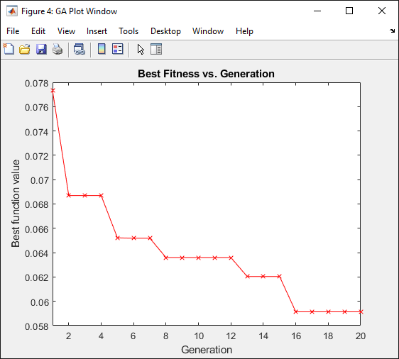
Best Fitness Plot

The Best Fitness + RMS plot adds to this a plot of the RMS error for the best design in each generation. This additional information may be of interest if the user would like to know if the algorithm is trading model fidelity for smaller design changes. In that case, the objective function value could go down while the RMS error increases. If this does happen and the user is more interested in reducing the RMS error, then the user should probably lower individual or global design weights.

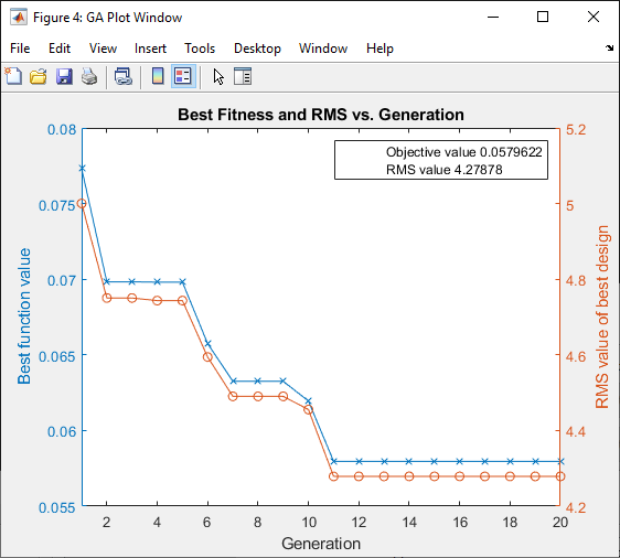
Best Fitness + RMS Plot

The Diversity plot gives insight into the degree of diversity in the “genes” which make up the designs being considered by the GA. As the optimization proceeds, the gene pool will likely become more homogeneous, containing the elements of designs which improve the objective function. This effect is countered by the mutation rate, which throws random elements into the gene pool to ensure that the design space is properly explored. If the diversity plot shows little range in objective function values, there is probably little more that the GA can do with further iteration unless mutation brings in new design possibilities.

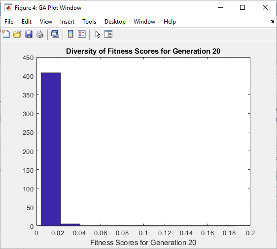
Diversity Plot

The Best Design plot shows the actual design values for the best design for each generation. It can be useful to watch the evolution of the best design. If the best design undergoes significant changes with each generation, then the user may question whether the solution has converged or whether some variables are changing because they have very little sensitivity. It can also be instructive to see how close to the bounds design variables are tending. If the design variables tend to be close to the bounds, the user may reconsider the bounds or rerun Nastran with the design variable set closer to the bounds to get a better estimate of the sensitivities. The plot also shows the bounds and limits to give the user an idea where the design fits within the specified bounds. A green line marks the initial design variable value. A blue bar shows the change in the design variable value for active design variables (a dark gray bar is used for inactive design variables). The limits established by the limit field on the Design Variable form are depicted as a white box. If no limit was set, the box extends to the upper and lower axis limits. The upper and lower bounds are depicted as gray bars with hatching. If no bounds were provided for a design variable, there would be no gray, hatched box for that design variable in the plot. The effective bounds are visually displayed as the area within the white box that is not overlaid with the light gray box. If the user changes the effective bounds on the GA form, the plot will reflect this by showing the limits and bounds as being equal to the effective bounds.

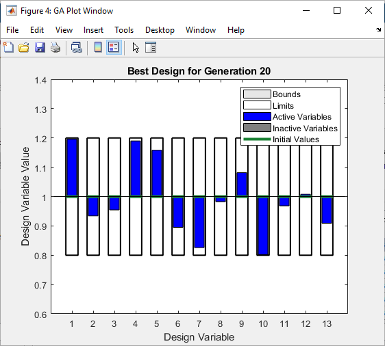
Best Design Plot

The Range plot shows the best, worst, and mean objective function value for each generation. The best and mean are plotted against the axis on the left. The worst values are plotted against the axis on the right. This plot does give some indication of the diversity of the gene pool. As the optimization converges, the mean value will approach the best value. The worst value will likely not converge because mutation usually introduces at least a few outliers in each generation.

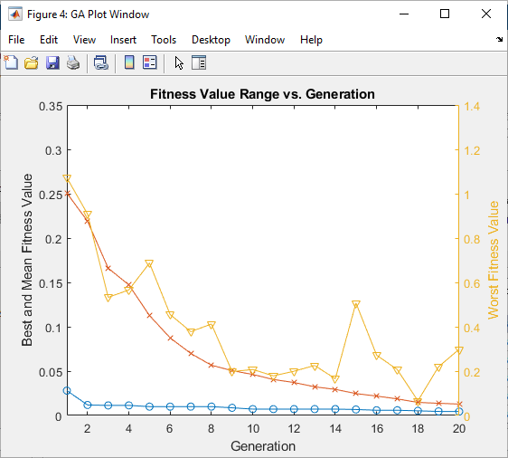
Range Plot

The Scores plot is a scatter plot of all objective function values for a particular generation. This plot gives another view of the diversity of objective function values for a given generation. As the optimization converges, the range of values in this plot should decrease.

Scores Plot