Demo
An example problem is presented in this section to show how to use Attune as part of the test-analysis correlation process. The overall correlation process consists of the following steps:
Normal modes analysis for baseline model
Comparison of baseline model with test and creation of design variables
Sensitivity analysis
Optimization of model updates based on sensitivities
Creation of a final updated model for normal modes analysis
Comparison of updated model with test
Typically, the sensitivity analysis and optimization are repeated until satisfactory agreement is obtained between test and analysis. The final model, called the test-validated model, accurately predicts the test results. The example problem analyzes a general purpose model (GPM) satellite using Nastran and Attune. Frequencies and cross-orthogonality are used as state variables.
Example Overview
This example problem illustrates the standard steps required to use Attune for test-analysis correlation. The example problem consists of a simple FEM of a satellite shown below. The baseline version of the model represents the “pretest” model. A similar version of the model with modified properties provides the test results for comparison. The pretest and test properties are shown in the table.
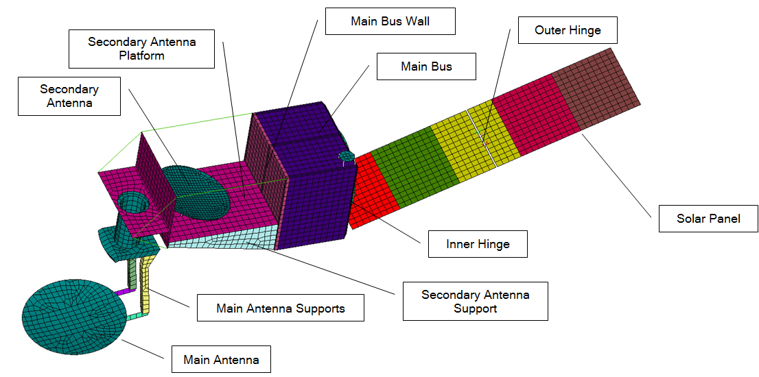
General Purpose Satellite Model
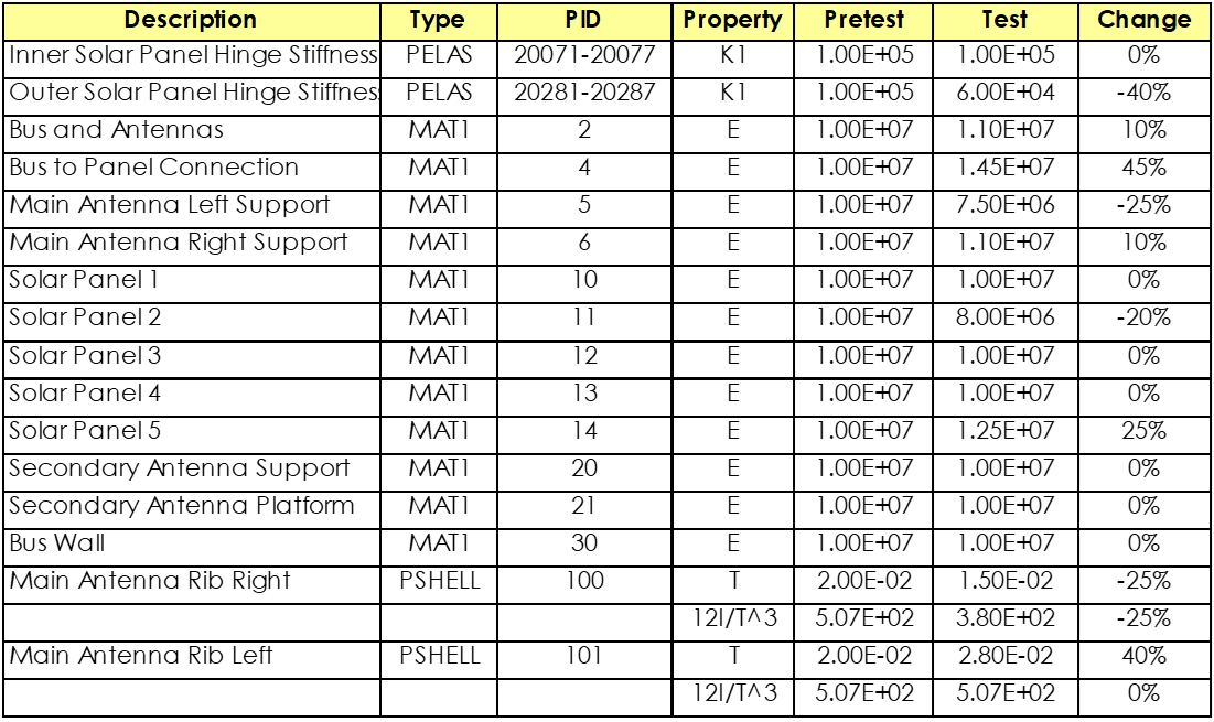
Test and Pretest Properties For Demo
Initial Configuration Creation
At the start of a typical correlation, a configuration must be created that contains all the required data. In this case, the analysis data, the test data, and the node mapping between the two models is required.
To start, the SOL 103 data is loaded into Attune. This is the starting point of the correlation – it will establish baseline frequency and shape errors, and allow the user to compare mode shapes. This is accomplished by selecting the folder icon on the Shape File in the Analysis Data panel while the Active Data Set is set to Pre-Optimization. Attune will ask if it is okay to load in the bulk data as well. Once this is done, the tab will appear like below. The pre-opimization analysis data is now loaded, so design variables can be created, as described in the next section.
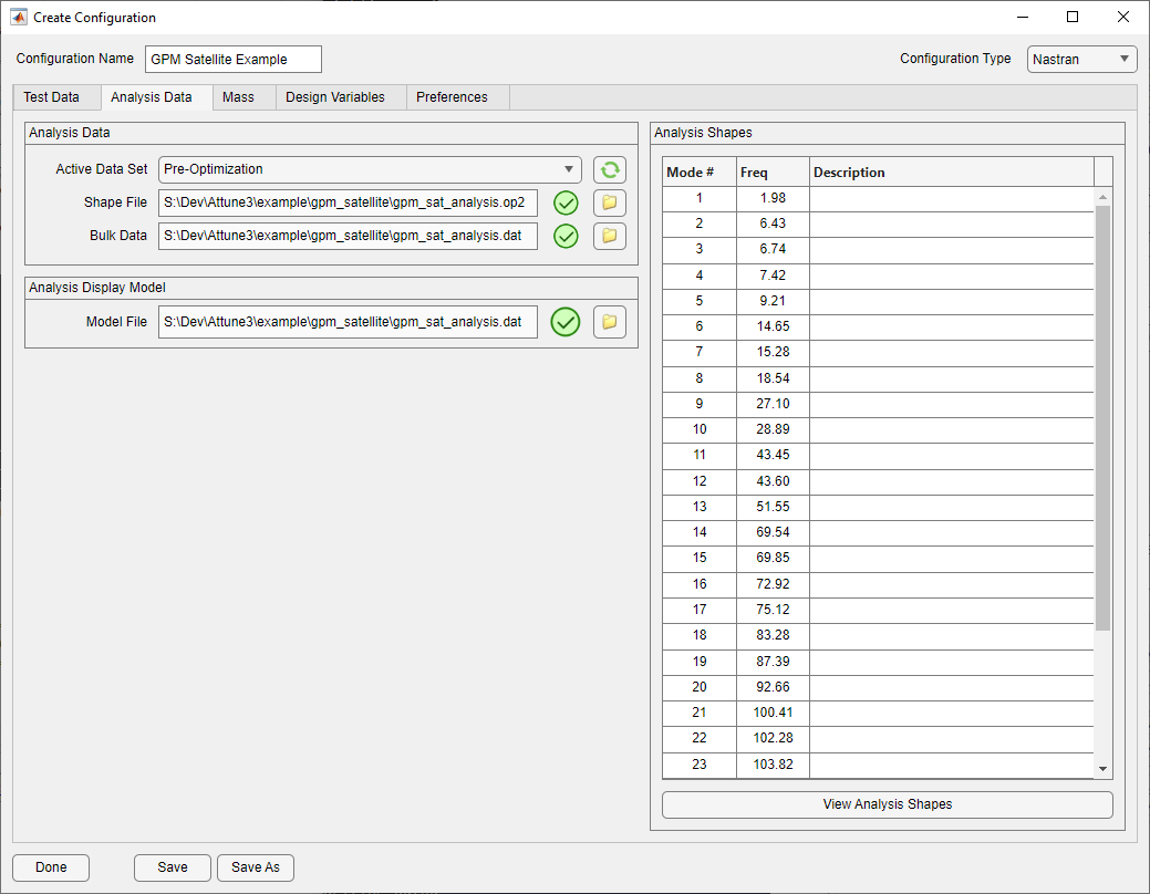
Analysis Data Loaded
Before that is done, however, test data should be read in. This is done by selecting the folder icon next to Test Shapes and selected the file that contains the test shape. The test display geometry is loaded in a similar way by selecting the requisite file after pressign the load button next to Test Geometry. Loading the test geometry allows the mode shapes to be visualized, and provides the input to the node mapping so the shapes can be related if their underlying node IDs are not identical.
Once the test model and analysis model geometry are loaded, check the Mapping Required from Test Geometry to Bulk Data to activate the mapping panel. The green checkmarks confirm that the required data has already been loaded and Create Map can be pressed to start the mapping process, as shown below.
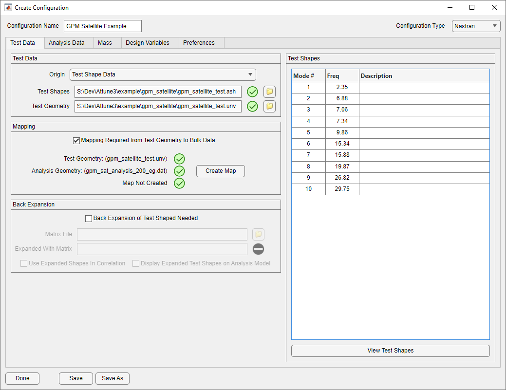
Test Data Loaded
After the Create Map button is pressed, the Node Mapping form is created. Again, because the test nodes and analysis nodes of the example model are not consistently numbered, a mapping needs to be created so that the test shapes and analysis shapes can be accurately compared. A mapping is created by pressing the Auto Match button. Since this example has simple geometry, it was possible to create a complete mapping by simply auto-matching. In the case where matches for some test nodes were not able to be found, matches can be made manually by using the Assign button or by using matches suggested by the List Closest Nodes button. The Mark Problems button will highlight any test nodes that do not already have a match. If any nodes remain unmatched, the test shape will be truncated. The form after the mapping is completed is shown below.
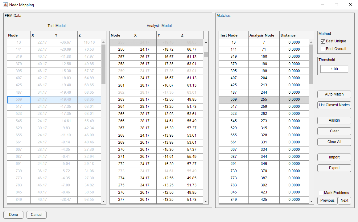
Test and Analysis Models Mapped
Design Variable Creation
After the test and analysis data has been loaded into the Pre-Optimization Data Set, it is time to begin the process of creating design variables and a SOL 200 deck. This is done by clicking on the Design tab at the top of the Configuration Creation form. From this tab, the user can create and set up design variables and write out a SOL 200 file. In this case, the correlation started from a SOL 103 analysis, so the design tab is initially blank. If the configuration is started from a SOL 200 file, or the configuration is edited later the Design tab will be prepopulated with the design variables from the bulk data.
The configuration form with design variables created is shown below.
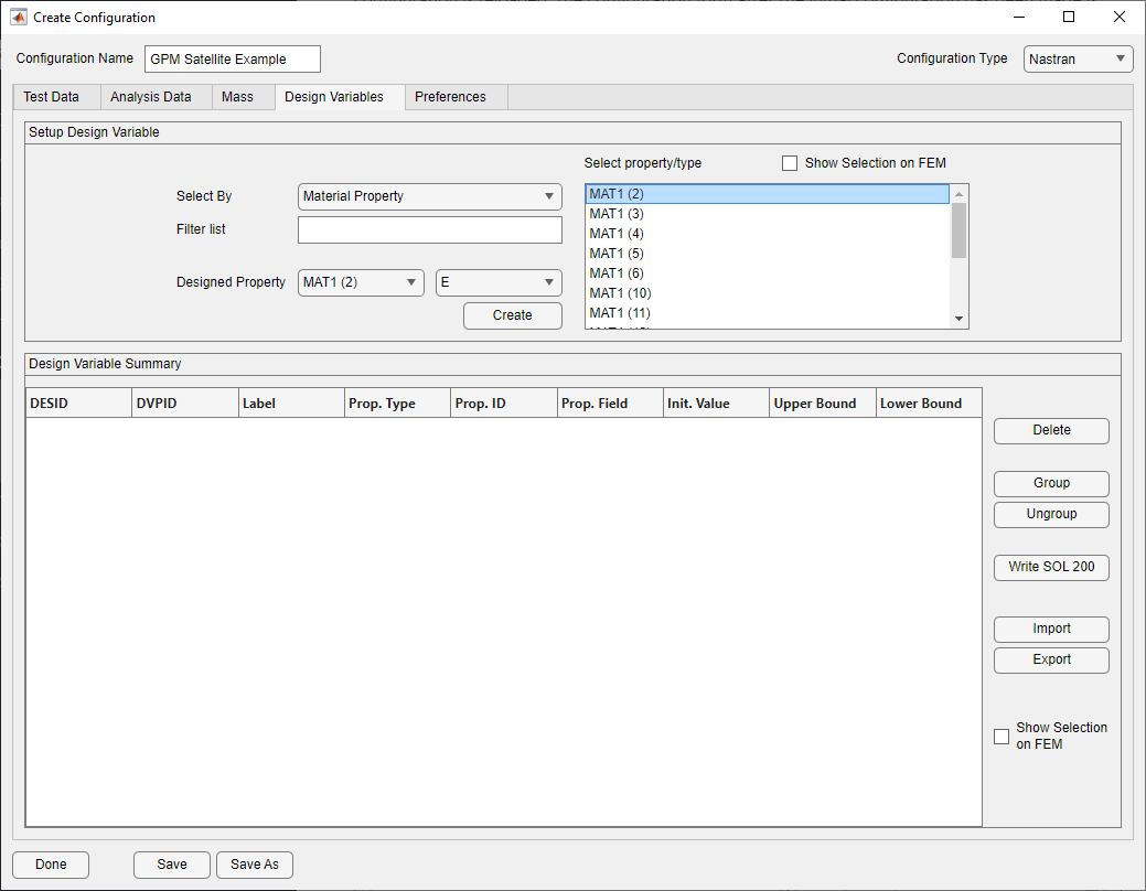
Initial Design Tab
Design variables are created by using the Setup Design Variable panel. This panel contains useful tools for setting up the material or physical properties to use for design variables. The Select By pulldown changes the manner in which the properties are selected. For this example, design variables will be created by selecting by Material Property and Physical Property. These two options are the simplest way of creating design variables, as the listbox simply contains a list of all of the material properties or all of the physical properties, respectively. The other options are discussed in detail in the Configuration Creation Form section under Getting Started.
After the Select By method is chosen, the desired property is selected from the listbox. Once this has been done, the Designed Property pulldowns will populate. The left pulldown lists the selected property/material and any related properties. The right pulldown lists designable fields of the property/material selected in the left pulldown. In the figure above, a MAT1 with ID 2 is selected, indicating that the user wishes to create a design variable that will vary Young’s modulus. Once the values in the pulldowns are set as desired, pressing Create will create the design variable and add it to the table.
Once a design variable is added to the table, it can be manipulated further. This includes changing the design variable (DESVAR) ID, the design variable property relation (DVPREL1/DVMREL1/DVCREL1) ID, the design variable label, the initial value, and the upper and lower bounds on the design variable. If the user desires to group design variables, the user can select them from the table and click Group. Conversely, grouped design variables can be ungrouped by pressing the Ungroup button. Grouped design variables will be constrained to vary together using one DESVAR. By ungrouping, the design variables are allowed to vary individually according to their own DESVAR.
In this example, design variables were created for the inner and outer joints of the solar panel, the ribs for the main antenna, the supports for the main antenna, the stiffnesses of the five individual panels that make up the solar panel, as well as the support structure for the secondary antenna. Because the analysis model has four springs to represent each joint of the solar panel, these design variables were grouped together.
The form after the design variables have been created is shown below.
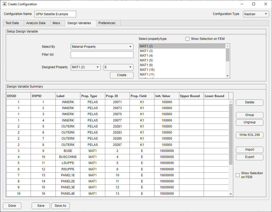
Design Tab with Design Variables Created
After the design variables are created, they are written out by pressing the Write SOL 200 button. A dialog appears asking for a name for the root Nastran file. A name other than the name of the SOL 103 file is required. Afterward, another prompt asks what suffix should be appended to included files, should they need to be updated as well. Any new cards that are required for a Nastran design optimization are automatically inserted into the root file.
After solving the SOL 200 deck in Nastran, the new data is read in by returning to the Analysis Data tab, switching the Active Data Set to Optimization and then loading in the file like was done for the SOL 103 shapes. Each configuration can store analysis data for the initial SOL 103 model (Pre-Opimization), the SOL 200 model with design variables (Optimization), and the resulting SOL 103 model after the properties are updated with the optimal design (Post-Optimization). The configuration can be switched between the three sets of data, and the main form will react accordingly with the parts of Attune that are relevant for the selection. If there are multiple configurations, they all must be set to the Optimization data set to be able to continue the correlation.
Comparison of Test and Analysis
Whenever a configuration is saved and Attune has a corresponding set of test and analysis data, it tries to identify matches between the test and analysis shapes based on cross-orthogonality. Once the matches are identified, Attune creates frequency and cross-orthogonality state variables. The figure below shows Attune’s main interface after the test and analysis data have been read in and the configuration created.
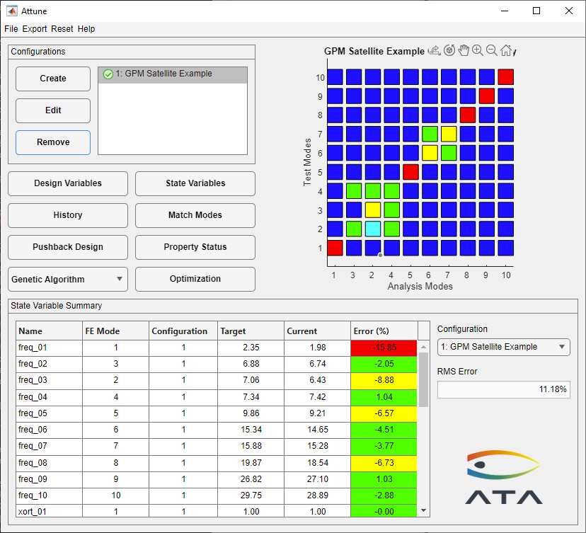
Main Form After Initial Configuration Created
The figure below shows the State Variable form indicating that the RMS error for the state variables is 11.2%. The cross-orthogonality and frequency comparison for the initial design are shown in the table. The initial mass properties are assumed to be the target values.
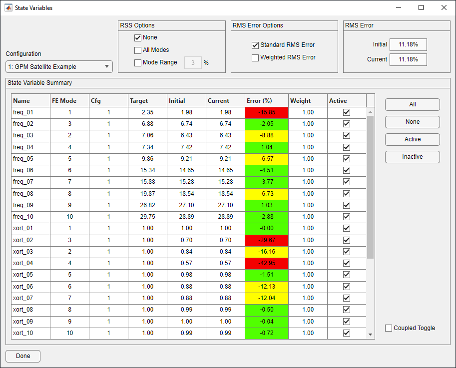
State Variable Form For the Initial Design
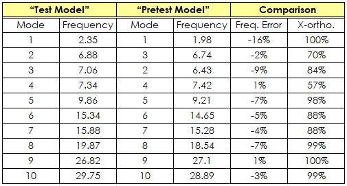
Initial Comparison of “Test” and “Pretest” results
Preparing for Optimization
Before running the optimization, the limits on the design variables must be set. The Design Variable form for the GPM satellite is below. Note that the limits for all variables have been set to ± 50%. This is a larger design space than for the typical model: the size of the design space is governed by the values over which the analyst believes the sensitivities to be valid and the expected error in property values. In this example, the expected error is high and the region over which the sensitivities are valid is fairly large (learned from experience with the model). It is also important to note that the design variable bounds could have also been set when creating the SOL 200 deck on the configuration form. It is a matter of preference and foresight as to whether or not the bounds are defined when creating the configuration or when preparing for the optimization.
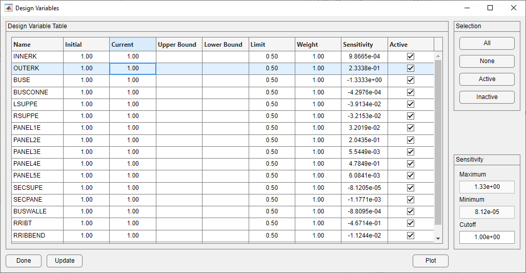
Initial Design Variable Form With Limits Set
The Design Variable form with a sensitivity cutoff is shown below. The design table shows the relative sensitivity of the model to the design variables. For this example, a cutoff of 1.0e-4 was used. This cutoff results in one variable, SECSUPE, becoming inactive. It is useful to make insensitive design variables inactive. Allowing them to vary expands the design space without contributing useful information and is likely to provide misleading results.
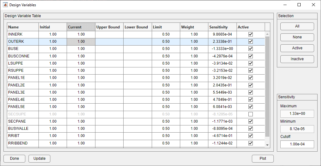
Initial Design Variable Form With Sensitivity Cutoff Used
Optimization
Now that the design variable limits and weights have been set, it is time to determine the optimal model update. Clicking the Optimization button on the main form with the Genetic Algorithm option selected brings up the GA Optimization form. It is a good idea to review the population size and the number of generations to make sure that they are set appropriately. For this example, the default GA settings are acceptable. To make certain that the best design always remains in the design population, the number of elite children will be set to one.
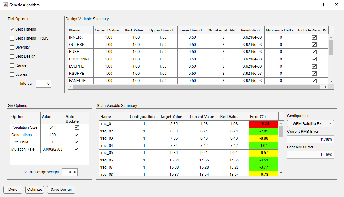
Genetic Algorithm Form with Default Settings
The optimization is initiated by pressing the Optimize button. The improvement in objective function value of the best design in each generation is shown below in the Best Fitness vs. Generation plot. Notice that the objective function value improves monotonically. This occurs whenever elite children are used. Without elite children, the objective function value may degrade over a few generations because the best design did not survive crossover and mutation. After optimization is completed, as shown below, notice that the overall RMS error has been reduced from 11.2% to 0.683%. The improvement in the solution can also be seen on the main form, also shown below. Note that the off-diagonal elements of the cross-orthogonality matrix visible in the initial design have been significantly reduced.
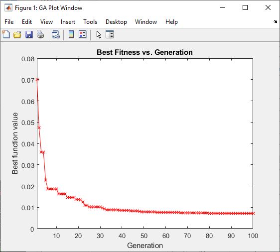
Objective Function Value Plot For Best Design in Each Generation
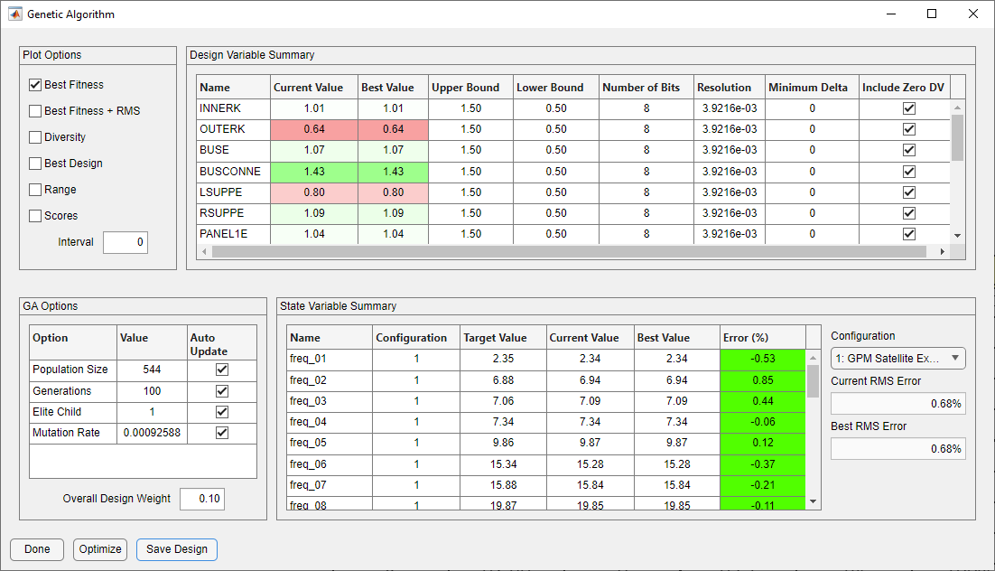
Genetic Algorithm Form After Optimization Complete
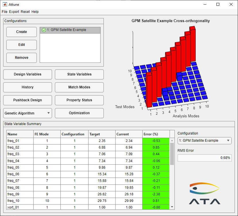
Attune Main Form After Optimization Complete
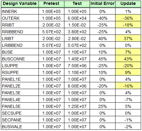
Comparison of Correlation Status After One Iteration
The table above contains the list of design variables and compares the “pretest” and “test” designs with the update suggested by Attune. Note that Attune correctly identified eight out of ten parameters with significant design changes, highlighted in yellow in the table. The parameters that Attune did not identify are the bending stiffness of the right rib and the stiffness of solar panel 5. The bending stiffness is highly coupled with the thickness of the rib and is difficult to identify because it has lower sensitivity than the thickness. The stiffness of panel 5 also has little sensitivity.
It is also important to note that Attune also updated some variables that did not have design changes. This, however, is not a flaw of Attune. The majority of these design variables had low sensitivity, as was seen on the Design form. This means that a large design change would cause a small improvement to the objective function. Since their sensitivity is low, these design variables tend to wander during the optimization. This is why it is important to disable design variables with low sensitivity, run multiple iterations in Attune, and use the Pushback Form. Because Attune uses a linear approximation to predict design changes, if the path to the correct design is very nonlinear, it is possible that Attune will either overpredict or underpredict the required design update. Moreover, writing the design out to Nastran will allow Attune to recalculate the linear approximation of sensitivities about an improved design and most likely cause the erroneous wandering to correct itself.
The sensitivities in the Design Filter form after the optimization is complete are shown below to demonstrate that there is significant dependence of the sensitivities on the current value of the design variables. Some variables’ sensitivities have changed by more than an order of magnitude.
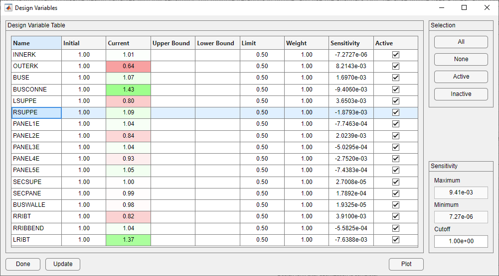
Design Form After First Iteation
The table below compares the improvement predicted by Attune to the actual improvement achieved by running the new design in Nastran. The predicted errors in frequency are very close to the actual errors, with a maximum of 1.79% difference between predicted and actual frequency. The cross-orthogonality predictions match the actual cross-orthogonalities uniformly well. Note that the modes which started out in reverse order (modes 2 and 3) now appear in the correct order.

Comparison of Predicted Design Improvement vs. Actual
This is only one iteration in the model-updating process. In this case, the results have improved dramatically in just one iteration, with almost “perfect” mode shapes and a maximum 3% frequency error. This is largely a phenomenon of this very simple example and is rarely encountered in practical correlation problems.
To document the correlation results of this iteration as XML files, select Current Design to Spreadsheet from the Export menu on the main form. This will produce an Excel XML document showing the status of the correlation. If this file is overwritten as the correlation process continues, Attune will append results to the existing file. Each time the file is written, the current status of the correlation is added to the summary sheet and two sheets are added containing a full description of the current state and design, respectively. The summary, state, and design tabs of the spreadsheet are shown in the figures below.
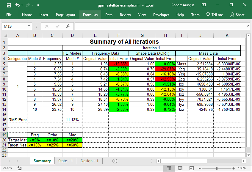
XML Correlation Summary After One Iteration
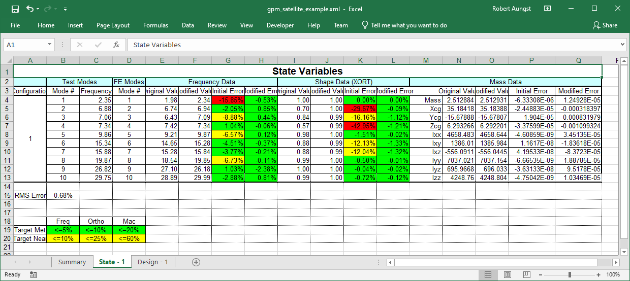
XML State Variable Status After One Iteration
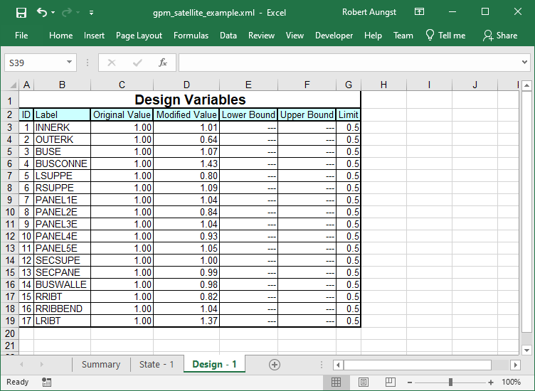
XML Design Variable Status After One Iteration
To continue the correlation process, the design suggested by Attune is written to the Nastran bulk data in a form that is ready to run. The figure below shows the form brought up by selecting Current Design Variables to Nastran Bulk from the Export menu on the main form. In this case, all design variable definition cards are in the same bulk data file. This is not required. Once the new design has been written out, Nastran is rerun and the configuration can be reloaded by selecting the Reload All Configurations item under the File menu on the main form. This action will reload the test data and the recently updated analysis data, remap the nodes, and update Attune with the new information.
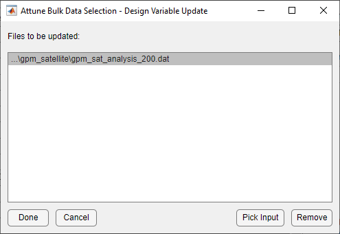
Bulk Data Selection Form For Updating Design Variable Values
After multiple iterations of Attune, when a satisfactory design is found, the final design can be written to a Nastran input file by selecting Final Property Values to Nastran Bulk from the Export menu on the main form. This will update the physical and material properties in the bulk data with the values indicated by the design variables. All Nastran parameters and design variables related to design optimization will be commented out, and the deck will be converted to SOL 103.
The new set of data is added to Attune by editing the configuration, changing the Active Data Set to Post-Optimization and loading in the final SOL 103 shapes. Upon saving the configuration and returning to the main Attune form, it will look like the figure below. The final status of the state variables is also shown below.

Main Form Showing Final Design After Writing Final SOL 103
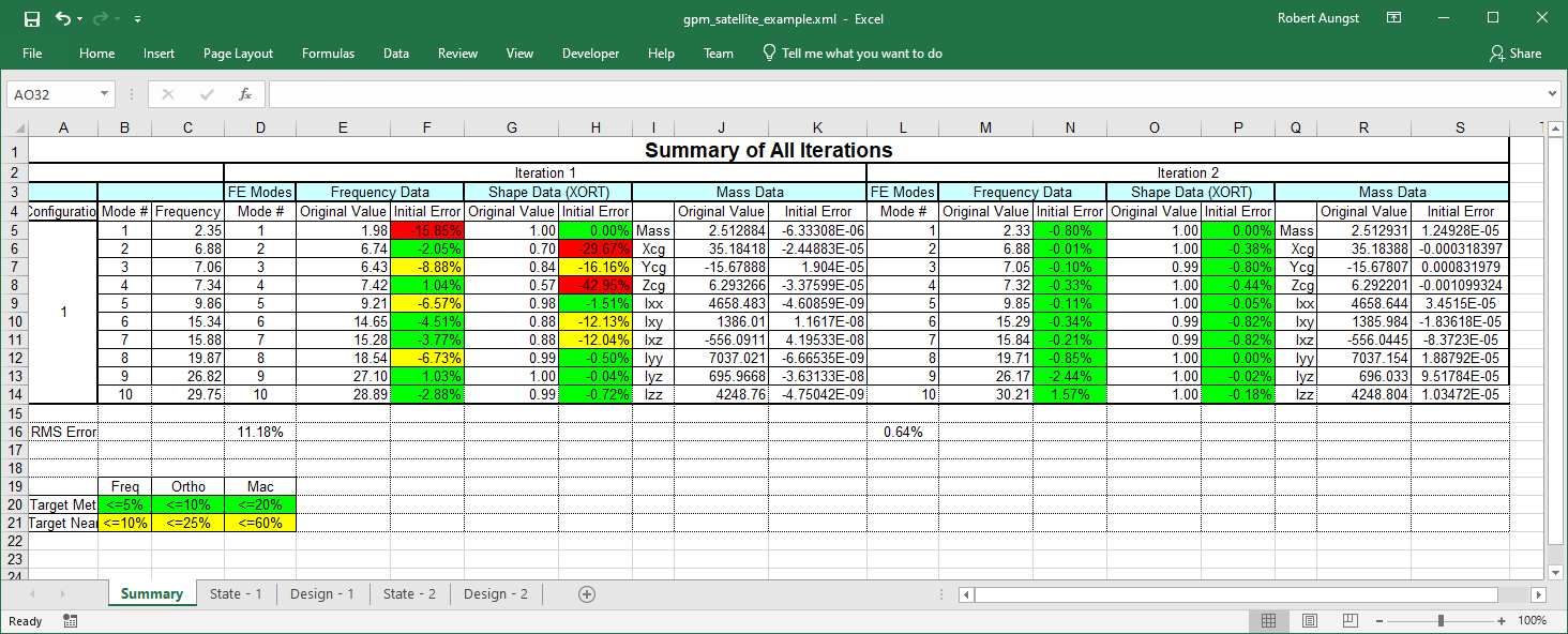
Final XML Output Showing Progress of Correlation